Joint and combined variation describe relationships where multiple variables change simultaneously according to specific mathematical rules. Joint variation occurs when a variable varies directly with the product of two or more other variables, while combined variation involves a mix of direct and inverse variations within a single expression. Understanding these concepts allows for accurate modeling of complex real-world scenarios in fields such as physics, economics, and engineering.
Understanding Joint and Combined Variation
Joint variation occurs when a variable depends on the product of two or more variables. Combined variation involves both direct and inverse variations within a single expression.
Understanding these concepts helps solve problems where multiple factors influence an outcome simultaneously. Formulas like z = kxy (joint) and y = kx / z (combined) illustrate their applications clearly.
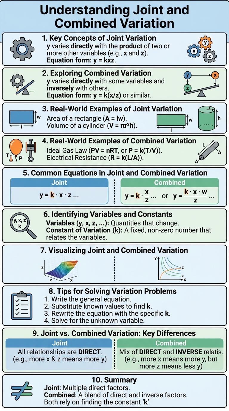
Key Concepts of Joint Variation
What is joint variation in mathematics? Joint variation describes a relationship where a variable depends directly on the product of two or more other variables. It is represented by the formula z = kxy, where k is the constant of variation.
How does combined variation differ from joint variation? Combined variation involves a variable that varies jointly with some variables and inversely with others. The general form is z = k (xy) / w, showing direct variation with x and y and inverse variation with w.
Exploring Combined Variation
Joint and combined variation describe how variables change relative to each other in mathematical relationships. Combined variation involves multiple types of variation simultaneously impacting an outcome.
- Joint Variation - One variable varies directly as the product of two or more other variables, expressed as z = kxy.
- Combined Variation - A variable varies directly with one variable and inversely with another, such as y = kx/z.
- Applications - Combined variation models real-world scenarios where factors multiply and divide to affect results, aiding problem-solving in physics and economics.
Real-World Examples of Joint Variation
Joint variation occurs when a variable depends on the product of two or more variables. Combined variation involves variables that vary jointly with some and inversely with others.
- Physics - Gravitational Force - The gravitational force between two masses varies jointly with the product of their masses and inversely with the square of the distance between them.
- Economics - Cost Calculation - The total cost of production varies jointly with the number of units produced and the cost per unit.
- Engineering - Pressure in Fluids - Pressure varies jointly with fluid density and gravitational acceleration and inversely with the height of the fluid column.
Real-World Examples of Combined Variation
| Example | Description |
|---|---|
| Physics: Gas Pressure | Pressure varies jointly with temperature and inversely with volume, modeling combined variation with P = k(T/V). |
| Economics: Revenue Calculation | Revenue varies jointly with price and quantity sold, and may vary inversely with discount rate. |
| Engineering: Force in Structures | Force exerted can vary jointly with acceleration and mass, showing combined variation in mechanics. |
| Biology: Population Growth | Growth rate varies jointly with birth rate and resource availability, combined with inverse variation by predation intensity. |
| Travel: Work-Schedule Relationship | Time taken for a trip varies jointly with distance and inversely with speed, a real-life example of combined variation. |
Common Equations in Joint and Combined Variation
Joint variation occurs when a variable depends on the product of two or more other variables. Combined variation involves a variable that varies jointly with some variables and inversely with others.
Common equations for joint variation take the form \( z = kxy \) where \( z \) varies jointly with \( x \) and \( y \). In combined variation, equations often look like \( z = \frac{kxy}{w} \), showing joint variation with \( x \) and \( y \) and inverse variation with \( w \).
Identifying Variables and Constants
Joint variation describes a situation where a variable depends on the product of two or more other variables, expressed as \( z = kxy \), where \( k \) is a constant. Combined variation involves a variable that varies jointly with some variables and inversely with others, such as \( z = \frac{kxy}{w} \). Identifying variables means recognizing the quantities that change, while constants are the fixed numbers that define the proportional relationship.
Visualizing Joint and Combined Variation
Joint and combined variation describe how variables change together in mathematical relationships. Visualizing these variations helps in understanding dependency and predicting values effectively.
- Joint Variation - Occurs when a variable depends directly on the product of two or more variables, such as z = kxy.
- Combined Variation - Involves a mix of both direct and inverse variation, like z = kx/y.
- Graphical Representation - 3D surface plots or contour maps clearly illustrate how variables interact in joint and combined variation.
Visual tools clarify how changes in one variable affect the others in joint and combined variation models.
Tips for Solving Variation Problems
Understanding the relationship between variables is key to solving joint and combined variation problems effectively. Identify whether the problem involves direct, inverse, or a combination of variations to set up the correct equation. Use consistent units and substitute known values carefully to find the unknown.